Machine Learning Models Basic Performance Metrics

You’ve collected some data and want to analyze it using machine learning, what do you do? What do you need to know? Other than just wanting to use machine learning, does it make sense to use machine learning?

Models

Classifier and regression models are two distinct types of machine learning models used for different types of tasks. Classifier models are used for classification tasks, where the goal is to predict the class or category of a given input instance. Heads versus Tails, red, green or blue, “one” or “zero”, these are example of classes. The input data in classification tasks consists of features or attributes, and the output is a discrete class label. Classifier models learn from labeled training data and aim to generalize patterns to make predictions on unseen data. Examples of classifier algorithms include logistic regression, decision trees, random forests, support vector machines (SVM), and neural networks. The performance of classifier models is typically evaluated using metrics such as accuracy, precision, recall, F1 score, and area under the ROC curve.

Regression models, on the other hand, are used for regression tasks, where the goal is to predict a continuous numeric value or a numerical target variable. In regression tasks, the input data also consists of features or attributes, but the output is a continuous value rather than a class label. Regression models learn from labeled training data to establish relationships between the input features and the target variable. Examples of regression algorithms include linear regression, polynomial regression, decision trees, random forests, and gradient boosting. The performance of regression models is often evaluated using metrics such as mean squared error (MSE), mean absolute error (MAE), and R-squared.

The main difference between classifier and regression models lies in the type of output they produce. Classifier models predict discrete class labels, while regression models predict continuous numerical values.

With the data collected you create a machine learning model and now you want to know how well the model performs. How is it measured? This blog explains some basic information and metrics to consider to help answer your question.

Metrics used to evaluate the performance of machine learning models include:

• Accuracy: The proportion of correct predictions out of the total number of predictions.
• Precision: The proportion of true positive predictions out of the total number of positive predictions, indicating the model's ability to avoid false positives.
• Recall: The proportion of true positive predictions out of the total number of actual positives, indicating the model's ability to identify all positive instances.
• F1 score: The harmonic mean of precision and recall, providing a balanced measure of a model's performance.
• Area Under the ROC Curve (AUC-ROC): A metric used for binary classification problems that measures the model's ability to distinguish between positive and negative instances across various probability thresholds.
• Mean Absolute Error (MAE): The average absolute difference between the predicted and actual values, commonly used for regression problems.
• Mean Squared Error (MSE): The average squared difference between the predicted and actual values, also commonly used for regression problems.
• R-squared (R2): A statistical measure that indicates the proportion of the variance in the dependent variable that can be explained by the independent variables.

The choice of metrics depends on the specific problem, the nature of the data, and model used.

In this paper we discuss the use ofclassification models. These models use accuracy, precision, recall, F1 score, specificity and AUC-ROC as metrics

These metrics provide insights into different aspects of a classifier's performance, such as overall accuracy, ability to classify positive instances correctly (precision), ability to capture all positive instances (recall), and the trade-off between precision and recall (F1 score). The choice of metrics depends on the specific problem and the evaluation criteria that are most important for the application at hand.

Accuracy

Accuracy is a metric used to measure the performance of a model in correctly predicting the labels or classes of the input data. It is calculated as the ratio of the number of correct predictions to the total number of predictions made by the classifier.

Mathematically, the accuracy (ACC) is defined as:

ACC = (Number of Correct Predictions) / (Total Number of Predictions)

In other words, accuracy represents the proportion or percentage of instances in the dataset that the classifier classified correctly.

Accuracy is a commonly used evaluation metric, especially in balanced datasets where the classes are represented fairly equally. However, accuracy alone might not provide a complete picture of a classifier's performance, especially in cases of imbalanced datasets where the number of instances in different classes is significantly different. In such cases, other metrics such as precision, recall, and F1 score might be more informative.

Precision

Precision is a metric that measures the proportion of true positive predictions out of the total number of positive predictions made by the classifier. It quantifies the model's ability to avoid false positive predictions. It measures the accuracy of positive predictions. Precision is also known as Positive Predictive Value.

Mathematically, precision is defined as:

Precision = PPV = (True Positives) / (True Positives + False Positives)

Positive Predictive Value quantifies the reliability of positive predictions made by the model. It provides insights into the likelihood that a positive prediction is correct. A high PPV indicates a low rate of false positive predictions, meaning that the model is accurate in classifying instances as positive.

Positive Predictive Value is particularly useful in scenarios where minimizing false positives is crucial, such as identifying potential cases of disease, fraud, or anomalies. It complements other metrics like sensitivity (recall) and is often used in combination with them to evaluate the overall performance of a classifier.

In other words, precision calculates the ratio of correctly predicted positive instances to the total instances that the classifier labeled as positive.

Precision is particularly relevant in scenarios where the focus is on minimizing false positives. For example, in a spam email classifier, precision measures the proportion of correctly identified spam emails out of all emails predicted as spam. A high precision value indicates that the classifier has a low rate of falsely labeling non-spam emails as spam.

It is important to note that precision should not be evaluated in isolation and needs to be considered in conjunction with other metrics such as recall, accuracy, and F1 score to comprehensively assess the performance of a classifier.

Sensitivity

Sensitivity, also known as recall or true positive rate (TPR), is a metric that measures the proportion of true positive predictions out of the total number of actual positive instances in the dataset.

Mathematically, sensitivity is defined as:

Sensitivity = (True Positives) / (True Positives + False Negatives)

In other words, sensitivity calculates the ratio of correctly predicted positive instances to the total instances that are actually positive.

Sensitivity focuses on the classifier's ability to identify and capture positive instances accurately. It quantifies how well the model avoids false negative predictions, which are instances that are actually positive but predicted as negative by the classifier.

Sensitivity is particularly important when the cost of false negatives is high or when the detection of positive instances is crucial. For example, in medical diagnosis, sensitivity measures the proportion of correctly identified individuals with a specific disease out of all individuals who actually have the disease.

Sensitivity is often used in conjunction with other metrics such as precision, accuracy, and F1 score to evaluate the overall performance of a classifier, especially in scenarios where correctly capturing positive instances is of greater importance.

Specificity

Specificity is a metric that measures the proportion of true negative predictions out of the total number of actual negative instances in the dataset. It is also known as the true negative rate (TNR).

Mathematically, specificity is defined as:

Specificity = (True Negatives) / (True Negatives + False Positives)

In other words, specificity calculates the ratio of correctly predicted negative instances to the total instances that are actually negative.

Specificity focuses on the classifier's ability to correctly identify and exclude negative instances. It quantifies how well the model avoids false positive predictions, which are instances that are actually negative but predicted as positive by the classifier.

Specificity is particularly important when the cost of false positives is high or when correctly identifying negative instances is crucial. For example, in a fraud detection system, specificity measures the proportion of correctly identified non-fraudulent transactions out of all transactions that are actually non-fraudulent.

Specificity is often used alongside other metrics such as sensitivity, accuracy, precision, and F1 score to evaluate the overall performance of a classifier, especially in scenarios where correctly capturing negative instances is of greater importance.

True Positive Rate

True Positive Rate (TPR), also known as sensitivity or recall, is a metric used in machine learning classifiers to measure the proportion of true positive predictions out of the total number of actual positive instances in the dataset.

Mathematically, the True Positive Rate is defined as:

TPR = (True Positives) / (True Positives + False Negatives)

In other words, TPR calculates the ratio of correctly predicted positive instances to the total instances that are actually positive.

True Positive Rate focuses on the classifier's ability to correctly identify and capture positive instances. It quantifies how well the model avoids false negative predictions, which are instances that are actually positive but predicted as negative by the classifier.

True Positive Rate is particularly important when the cost of false negatives is high or when the detection of positive instances is crucial. For example, in medical diagnosis, the True Positive Rate measures the proportion of correctly identified individuals with a specific disease out of all individuals who actually have the disease.

True Positive Rate is often used in conjunction with other metrics such as precision, accuracy, and F1 score to evaluate the overall performance of a classifier, especially in scenarios where correctly capturing positive instances is of greater importance.

False Positive Rate

False Positive Rate (FPR) is a metric used in machine learning classifiers to measure the proportion of false positive predictions out of the total number of actual negative instances in the dataset. It quantifies the rate at which the classifier incorrectly labels negative instances as positive.

Mathematically, the False Positive Rate is defined as:

FPR = (False Positives) / (False Positives + True Negatives)

In other words, FPR calculates the ratio of incorrectly predicted positive instances to the total instances that are actually negative.

False Positive Rate is important in scenarios where the cost of false positives is high or when correctly identifying negative instances is crucial. It helps assess the model's ability to avoid false alarms or falsely labeling negative instances as positive.

False Positive Rate is often used alongside other metrics such as specificity and precision to evaluate the overall performance of a classifier, especially in situations where minimizing false positives is a priority. It complements the True Positive Rate (sensitivity) and is commonly utilized in binary classification tasks.

Accuracy vs Precision

Accuracy and precision are both metrics used to evaluate the performance of machine learning classifiers, but they measure different aspects of classification results:

Accuracy: Accuracy measures the overall correctness of predictions made by a classifier. It calculates the ratio of correctly predicted instances (both true positives and true negatives) to the total number of predictions.

Precision: Precision focuses specifically on the proportion of true positive predictions out of the total positive predictions made by the classifier. It quantifies the model's ability to avoid false positive predictions.

The key differences between accuracy and precision are:

• Accuracy considers all types of predictions (true positives, true negatives, false positives, and false negatives) and provides an overall measure of correctness, while precision only focuses on the positive predictions and evaluates the proportion of true positives.
• Accuracy takes into account both the positive and negative predictions, providing a broader assessment of the classifier's performance. Precision, on the other hand, provides insights into the classifier's ability to make accurate positive predictions and avoid false positives.

It's important to note that the interpretation and appropriate usage of these metrics depend on the specific problem, the class distribution, and the desired balance between minimizing false positives and false negatives.

Visualization tools

When evaluating classifiers, several visualization tools can be used to gain insights into their performance. Some commonly used visualization tools include:

Confusion Matrix

Confusion Matrix Heatmap: A heatmap representation of the confusion matrix provides a visual summary of the classifier's performance, highlighting the distribution of correct and incorrect predictions across different classes.

A confusion matrix is produced by comparing the predicted labels of a classifier to the true labels of the data. Here are the steps to create a confusion matrix:

• Obtain the true labels of the data: These are the actual labels representing the ground truth for each instance in the dataset.
• Make predictions with the classifier: Apply the trained classifier to the input data and obtain the predicted labels for each instance.
• Create a matrix: Set up a square matrix where the rows represent the true labels and the columns represent the predicted labels. The size of the matrix depends on the number of unique labels in the dataset.
• Populate the matrix: Count the number of instances that fall into each combination of true and predicted labels and update the corresponding cell in the matrix. This can be done by iterating over the data and comparing the true and predicted labels for each instance.
• Interpret the matrix: The resulting confusion matrix provides a tabular representation of the classifier's performance. It shows the number of instances classified correctly (true positives and true negatives) as well as the number of instances misclassified (false positives and false negatives).

Image 1 represents data with 4 classes that is passed to a classifier 

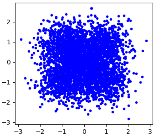
Table 2 is an example of a Confusion Matrix where there are 4 classes being predicted by the classifer. The data is well balanced between the classes. As you can see the diagonal has high numbers indicating the classifier is performing well.

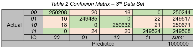
A confusion matrix helps to visualize and analyze the performance of a classifier by providing detailed information about its predictions and errors. It serves as a basis for calculating various performance metrics like accuracy, precision, recall, and F1 score.

AUC-ROC

ROC Curve: The Receiver Operating Characteristic (ROC) curve plots the true positive rate (TPR) against the false positive rate (FPR) at various probability thresholds. It helps assess the trade-off between sensitivity and specificity and can be visualized as a curve. The area under the ROC curve (AUC-ROC) is also a common metric to compare the performance of different classifiers.

image 2

Image 2 represents several models compared to each other using AUC curves. The The models are predicting a binary outcome with thousands of features. AUC performance is listed in the lower right legend.

Precision-Recall Curve

The precision-recall curve plots precision against recall at various probability thresholds. It helps evaluate the trade-off between precision and recall and can provide insights into the classifier's performance for imbalanced datasets.

Decision Boundary Visualization

For classifiers that operate in a feature space, visualizing the decision boundary can help understand how the classifier separates different classes. This can be particularly useful for classifiers that work with two or three-dimensional data.

Feature Importance Plot

For classifiers that incorporate feature importance analysis, plotting the importance scores of different features can provide insights into which features have the most significant impact on the classifier's predictions.

Error Analysis

Visualizing misclassified instances or exploring specific subsets of the data (e.g., false positives, false negatives) can help identify patterns or outliers that contribute to classification errors.

These visualization tools can aid in interpreting the classifier's performance, identifying areas for improvement, and gaining a deeper understanding of its behavior. The choice of visualization depends on the specific evaluation goals and the nature of the classifier and data.

Using Accuracy with imbalanced Data

Using accuracy as an evaluation metric with imbalanced data can be misleading and may lead to incorrect conclusions about the performance of a classifier. Dangers associated with using accuracy with imbalanced data can lead to Misrepresentation of performance. Accuracy does not account for class imbalance, so even a classifier that predicts only the majority class can achieve a high accuracy if the majority class dominates the dataset. This can create a false perception of a well-performing model when, in reality, it is not effectively capturing the minority class.

Imbalanced data leads to inadequate representation of minority class. In imbalanced datasets, the minority class can be of greater interest, such as detecting fraudulent transactions or rare diseases. Accuracy ignores the performance of the minority class.

In many real-world scenarios, misclassifying instances of the minority class (false negatives) may have more severe consequences than misclassifying instances of the majority class (false positives). Accuracy does not differentiate between these types of errors and treats them equally.

Imbalanced data can cause masking classifier bias. Accuracy may not reveal bias in the classifier's predictions. Even if the model predicts the majority class with high accuracy, it could be performing poorly on the minority class. Accuracy alone does not highlight potential disparities in performance across different classes.

To address these dangers, it is important to consider evaluation metrics that are more suitable for imbalanced datasets, such as precision, recall, F1 score, area under the ROC curve (AUC-ROC), or precision-recall curve. These metrics provide a more comprehensive understanding of a classifier's performance, especially when dealing with imbalanced data, by focusing on specific aspects like correctly identifying positive instances or managing the trade-off between precision and recall.

Evaluation of a Machine learning model

To determine if a machine learning model's predictions are better than random guesses, you can compare the model's performance metrics against the expected performance of random guessing. Here's how you can assess it:

Define a baseline: The baseline represents the performance of random guessing. It serves as a reference point for evaluating the model's predictions. For binary classification, random guessing would achieve an accuracy of 50% (randomly assigning labels to instances with equal probability).

Evaluate performance metrics: Calculate the relevant performance metrics for your model, such as accuracy, precision, recall, F1 score, or area under the ROC curve (AUC-ROC).

Compare against the baseline: Compare the model's performance metrics to the baseline. If the model's performance metrics are consistently better than the random guessing baseline, it indicates that the model is learning patterns and making predictions beyond random chance.

It's important to note that the choice of performance metrics depends on the problem and the evaluation criteria that are most important for your application. Some metrics, such as AUC-ROC or precision-recall curve, can provide more nuanced insights into a model's performance, particularly in cases of imbalanced datasets or when the trade-off between different evaluation measures is crucial.

Additionally, it's a good practice to use cross-validation or holdout validation techniques to ensure the model's performance is not biased by a particular train-test split.

Data with bias

When working with data that contains a high bias, it can be challenging to determine if a machine learning model's predictions are better than random guesses. However, you can still use certain approaches to assess the model's performance

Establish a baseline: Similar to the previous scenario, establish a baseline performance metric based on random guessing. For random binary data sets, random guessing would yield an accuracy of 50%, for example, outcomes of flipping of a coin. For 90% biased binary data sets guessing, could yield 90%.

Compare outcomes against the expected bias. Assess whether the model's predictions show improvement over the expected bias in the data. If the model performs better than the bias present in the data, it suggests that the model is capturing some meaningful patterns.

Use performance metrics that account for data bias. In cases of high bias, traditional performance metrics like accuracy will not provide a complete picture. Consider alternative evaluation techniques that focus on specific aspects, such as precision, recall, F1 score, or area under the ROC curve (AUC-ROC). These metrics can provide insights into the model's performance, especially when dealing with imbalanced data or biased scenarios.

It's important to note that assessing model performance in the presence of high bias can be complex and may require larger data sets. It requires careful interpretation of results, consideration of domain knowledge, and a thorough understanding of the limitations and biases in the data itself.

Common Metrics and definitions

TN = True Negative

FP = False Positive

FN = False Negative

TP = True Positive

AP = all positives = TP + FN

AN = all negatives = TN + FP

PP = predicted positives = TP + FP

PN = predicted negatives = FN + TN

Sensitivity, also known as recall (ability to find positive results) is the percentage of predicted true positives to all real positives,

sensitivity = TP / AP = TP / (TP + FN)

Specificity is the ability to find the true negatives.

specificity = TN / AN

Total number of samples being evaluated.

sample_size = AP + AN

Accuracy all correct predictions divided by sample size (all samples)

accuracy = (TN + TP) / sample_size

Prevalence is either all positives or all negatives (depending on which is higher) divided by all samples

Prevalence(P) = AP / sample_size

Prevalence(N)= AN / sample_size

Positive Predictive Value is ability of a classification model to return only relevant instances

PPV = TP / (TP + FP)

Positive predictive value, precision

PPValue = TP / PP

Negative predictive value

NPValue = TN / PN

F1score = 2*PPValue*sensitivity/(PPValue+sensitivity)

receiver operator characteristic curve area under the curve

roc_auc = auc(fpr, tpr)

Summary

When analyzing data using machine learning, you need to select a suitable model based on the task at hand.

Classifier models learn from labeled training data and predict discrete class labels, while regression models learn from labeled training data and predict continuous numerical values.

To evaluate the performance of machine learning models, various metrics can be used. These include accuracy, precision, recall, F1 score, area under the ROC curve (AUC-ROC) for classification models, and mean absolute error (MAE), mean squared error (MSE), and R-squared (R2) for regression models. The choice of metrics depends on the specific problem and the nature of the data.

Visualization tools such as confusion matrices, ROC curves, precision-recall curves, decision boundary plots, feature importance plots, and error analysis can be used to gain insights into the performance of classifiers and understand their behavior.

When dealing with imbalanced data, using accuracy as an evaluation metric can be misleading. Accuracy alone does not account for class imbalance and may overestimate the performance of a classifier, especially for minority classes. It is important to consider other metrics such as precision, recall, and F1 score, which provide a more comprehensive evaluation of classifier performance in imbalanced datasets.

Sign in